python数据拟合和分析

以下内容是我在进行webRTC拥塞控制部分进行训练集traces分析和生成的总结;举办方提供了一部分真实环境的数据,但我认为对于训练来说可能不够,因此需要自己生成一部分;

数据拟合

使用fitter库进行数据的拟合;大概的效果如下图所示:

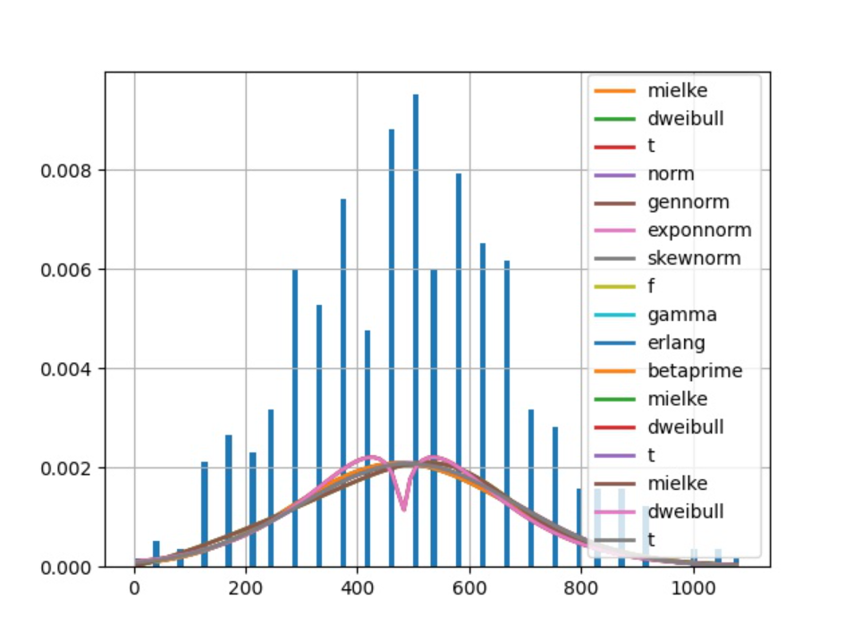
image-20210712190334719

fitter 库

fitter库的源码位置:https://github.com/cokelaer/fitter

安装fitter库: pip install fitter

fitter库的文档:https://fitter.readthedocs.io/en/latest/

fitter库使用案例

生成模拟数据:

1
2
3
>>> # First, we create a data sample following a Gamma distribution
>>> from scipy import stats
>>> data = stats.gamma.rvs(2, loc=1.5, scale=2, size=20000)

使用 fitter库进行拟合:

1
2
3
4
5
6
7
8
9
10
11
12
13
14
15
16
17
>>> # We then create the Fitter object
>>> import fitter
>>> f = fitter.Fitter(data)

>>> # just a trick to use only 10 distributions instead of 80 to speed up the fitting
>>> f.distributions = f.distributions[0:10] + ['gamma']

>>> # fit and plot
>>> f.fit()
>>> f.summary()
sumsquare_error
gamma 0.000095
beta 0.000179
chi 0.012247
cauchy 0.044443
anglit 0.051672
[5 rows x 1 columns]

它在使用fit函数的时候如果没有额外的参数会用scipy的80多个分布进行逐个拟合,默认的拟合时间是30秒;

fitter库参数

  1. fitter

    1
    class fitter.fitter.Fitter(data, xmin=None, xmax=None, bins=100, distributions=None, timeout=30, density=True)
    • data (list) –输入的样本数据;
    • xmin (float) – 如果为None,则使用数据最小值,否则将忽略小于xmin的数据;
    • xmax (float) – 如果为None,则使用数据最大值,否则将忽略大于xmin的数据;
    • bins (int) – 累积直方图的组数,默认=100;
    • distributions (list) – 给出要查看的分布列表。 如果没有,则尝试所有的scipy分布(80种),常用的分布distributions=[‘norm’,‘t’,‘laplace’,‘cauchy’, ‘chi2’,’ expon’, ‘exponpow’, ‘gamma’,’ lognorm’, ‘uniform’];
    • verbose (bool) –
    • timeout – 给定拟合分布的最长时间,(默认=10s) 如果达到超时,则跳过该分布。
    1
    2
    3
    4
    5
    6
    from fitter import Fitter
    # may take some time since by default, all distributions are tried
    # but you call manually provide a smaller set of distributions
    f = Fitter(data, distributions=['gamma', 'rayleigh', 'uniform'])
    f.fit()
    f.summary()
  1. 进行fitter了之后可以调用一下函数

    1
    2
    3
    4
    5
    6
    7
    8
    f.fit() #fit(amp=1, progress=False, n_jobs=-1)
    f.df_errors #返回这些分布的拟合质量(均方根误差的和)
    f.fitted_param #返回拟合分布的参数
    f.fitted_pdf #使用最适合数据分布的分布参数生成的概率密度
    f.summary() #返回排序好的分布拟合质量(拟合效果从好到坏),并绘制数据分布和Nbest分布 summary(Nbest=5, lw=2, plot=True, method='sumsquare_error')
    f.get_best(method='sumsquare_error') #返回最佳拟合分布及其参数
    f.hist() #绘制组数=bins的标准化直方图
    f.plot_pdf(names=None, Nbest=3, lw=2) #绘制分布的概率密度函数 plot_pdf(names=None, Nbest=5, lw=2, method='sumsquare_error')
  2. 使用注意点

    我在使用上述函数的时候f.hist()之后并没有出现图片,通过研究了它源码的issue发现比较保险的方法是import matplotlib,在 f.hist()之后加上plt.show()或者savefig()等操作,这样就能够显示图片了;

    1
    2
    3
    4
    5
    import matplotlib.pyplot as plt
    .....
    f.hist()
    plt.show()
    plt.close()

实际使用的脚本

1
2
3
4
5
6
7
8
9
10
11
12
13
14
15
16
17
18
19
20
21
22
23
24
25
26
27
28
29
30
31
32
33
34
35
36
37
38
39
40
41
42
# 批处理版
from __future__ import division
import json
import matplotlib as mpl
import matplotlib.pyplot as plt
import glob
import os
import numpy as np
from fitter import Fitter
f = glob.iglob(r'*.json') # 当前目录所有py文件,与glob区别,iglob每次只获取一个匹配路径
old_picture = glob.iglob(r'*.jpg')

result="最佳拟合分布"
for file in f:
with open(file, 'r') as f:
information=file+"\n"
trace_pattern = []
data = json.load(f)
data_intervals = data["uplink"]["trace_pattern"]
capacity = []
for ele in data_intervals:
capacity.append(ele["capacity"])
print("capacity_mean", np.mean(capacity))
capacity.sort()
length = len(capacity)
capacity = capacity[0:length-5]
filter1 = Fitter(capacity,distributions=["lomax","pareto","johnsonsu","exponweib","powerlognorm"])
filter1.fit()
print(type(filter1.summary()))
print(filter1.get_best(method='sumsquare_error'))
summary=str(filter1.summary())
information=information+"summary\n"+summary+"\n"
best_method=str(filter1.get_best(method='sumsquare_error'))
information=information+best_method
filter1.plot_pdf(names=None, Nbest=3, lw=2)
#plt.show()
plt.savefig("fit_{}.jpg".format(file))
plt.close()
result=result+"\n"+information
with open("fit_result.txt",'w') as f:
f.write(result)

效果是批处理如下json格式的数据,会统计一个文件夹中的数据,给每一个数据绘图,并且把summary写道fit_result.txt

1
2
3
4
5
6
7
8
9
10
11
12
13
14
15
16
17
18
19
20
21
22
{
"type": "video",
"downlink": {},
"uplink": {
"trace_pattern": [
{
"duration": 200,
"capacity": 0,
"loss": 0,
"jitter": 0,
"time": 0.0
},
{
"duration": 200,
"capacity": 0,
"loss": 0,
"jitter": 0,
"time": 0.0
}
]
}
}

数据折线图

1
2
3
4
5
6
7
8
9
10
11
12
13
import matplotlib.pyplot as plt

.....
plt.plot(time_x,time_capacity)
xlabels = ["{}".format(i) for i in time_x] #修改x轴的刻度
plt.xticks(time_x, xlabels)

plt.xlabel('row')
plt.ylabel('column')
plt.legend()
plt.savefig("time_{}.jpg".format(
file))
plt.close()

数据生成

经过查阅scipy的文档以及简单了看了fitter项目的源码,上面get_best()得到的形如:

1
'johnsonsu': (-0.43618926054816165, 1.8086581271068694, 26026.47774558232, 26854.12469365103)

表示的参数为a, b, loc, scale;

具体含义见下图:

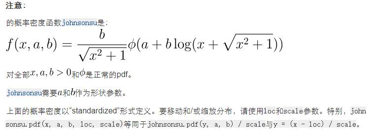
image-20210712190221706

通过上面fitter得到的参数,可以使用如下的代码进行数据的生成,生成的格式是narray:

1
2
3
4
import scipy.stats as st
size_t=1500
params=(-0.43618926054816165, 1.8086581271068694, 26026.47774558232, 26854.12469365103)
data=list(st.johnsonsu.rvs(*params,size=int(size_t))) # 格式是numpy

数据筛选

1
2
3
4
5
6
7
# 数据筛选
data1=data[:]
for ele in data1:
if ele < 0.0:
data.remove(ele)
if ele > 400.0:
data.remove(ele)

如果没有data1=data[:]的操作会出现无法删除的问题